How to Graph Absolute Value Functions

This lesson is about graphing an absolute value function when the expression inside the absolute value symbol is linear. It is linear if the variable “[latex]x[/latex]” has a power of [latex]1[/latex]. The graph of absolute value function has a shape of “V” or inverted “V”.

Absolute Value Function in Equation Form

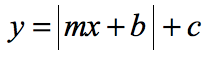
The general form of an absolute value function that is linear is

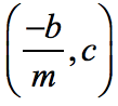
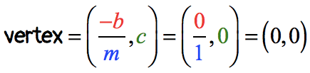
y is equal to the absolute value of mx+b plus c

where the vertex (low or high point) is located at

the vertical line

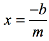
divides the graph into two equal halves

KEY POINTS TO REMEMBER:

The specific approach that we are going to use is to find the “right amount of points” that can be plotted on the [latex]xy[/latex]-axis so that we have a good approximation on how the graph of the absolute value function looks likes.

Don’t fall into the common trap to always use [latex]x = 0[/latex] as the middle value of the [latex]x[/latex] coordinates. This may work at times, but this idea is not so reliable.

I suggest using the [latex]x[/latex]-coordinate of the vertex, [latex]\left( {{{ – b} \over m},\,c} \right)[/latex], which is [latex]x = {{ – b} \over m}[/latex] as the middle value of all [latex]x[/latex]-values in the table.

In other words, once you have determined what the middle value for [latex]x[/latex] is, then go ahead and pick any arbitrary [latex]x[/latex] values to the left and right of it as long as it is properly spaced out.

Again, the best way to illustrate this simple idea is through the use of examples!

Examples of Graphing Absolute Value Functions

Example 1: Graph the absolute value function below using the table of values.

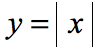
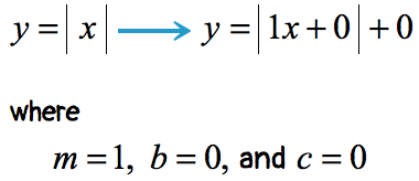
This is the most basic form of an absolute value function. If you see that the only expression inside the absolute value symbol is just “[latex]x[/latex]”, assume that the vertex of the graph will occur when [latex]x = 0[/latex].

Or, if you want to use the formula above to find the vertex, rewrite the given function in the standard form so that you can identify the values of [latex]m[/latex], [latex]b[/latex], and [latex]c[/latex].

y equals the absolute value of x implies y equals the absolute value of 1x+0 plus zero

The vertex is calculated as

Since [latex]x = 0[/latex], this becomes the center values of all [latex]x[/latex]’s. Now we can pick some numbers to the left and to the right of zero. I would suggest using equal amount of numbers that are of the same increment.

Pick [latex]-3[/latex], [latex]-2[/latex], [latex]-1[/latex] to the left of zero, and [latex]+1[/latex], [latex]+2[/latex], [latex]+3[/latex] to its right. Evaluate all values of [latex]x[/latex] into the function [latex]y = \left| x \right|[/latex] to get the corresponding [latex]y[/latex]-values.

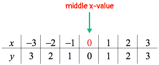
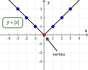
a horizontal table with a middle value of x of zero

Notice that the graph has a low point determined by the middle [latex]x[/latex]-value which is the [latex]x[/latex]-coordinate of the vertex itself, i.e. (0,0).

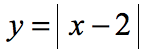
the graph of y=absolute value of x. it resembles a V shape and the vertex hits the origin or the point (0,0)

Example 2: Graph the absolute value function below using the table of values.

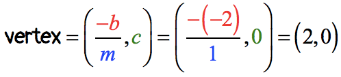
The first step is to find the [latex]x[/latex]-coordinate of the vertex which will serve as the center point in the table of values of [latex]x[/latex].

Rewrite [latex]y = \left| {x – 2} \right|\,\,\,[/latex]as [latex]y = \left| {1x + \left( { – 2} \right)} \right| + 0[/latex] where [latex] m = 1[/latex], [latex]b = -2[/latex], and [latex]c = 0[/latex]. We calculate the vertex as…

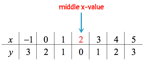
the vertex is at open paren 2 comma zero close paren or (2,0)

The [latex]x[/latex]-coordinate of the vertex will be the center value of all [latex]x[/latex]’s on the table. We generated the rest of the [latex]x[/latex] by finding three numbers to the left and right of the middle value of [latex]2[/latex] with an increment of [latex]1[/latex]. You may use an increment of [latex]2[/latex], and trust me, the graph will be the same.

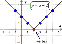
a sideway table where the middle x value is at x=2

Plot the points on the [latex]xy[/latex]-plane and connect the dots with a straight edge. If you get it right, you should have something similar below. As you can see, the low point of the graph is the vertex located at ([latex]2[/latex],[latex]0[/latex]).

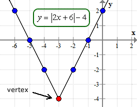
the graph of an absolute value function shifted two units to the right. the vertex is located at the point (2,0).

Example 3: Graph the absolute value function below using the table of values.

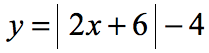
I hope you start realizing that the first step is to always express the given absolute value function in standard form. This allows us to identify the correct values of [latex]m[/latex], [latex]b[/latex], and [latex]c[/latex] which we will use to substitute into the formula.

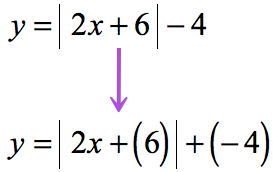
Clearly, the required values are [latex]m = 2[/latex], [latex]b = 6[/latex], and [latex]c = -4[/latex].

Then we calculate the vertex as follows;

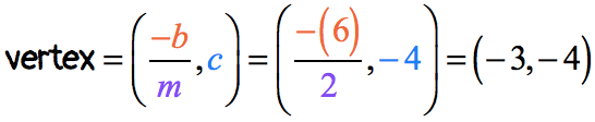
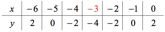
the vertex is located at the point negative 3 comma negative 4 or (-3,-4)

Our table of values will have a center value of [latex]x = – 3[/latex]. Generate 3 numbers both to the left and right of [latex]x = – 3[/latex] with an increment of [latex]1[/latex]. Then evaluate each value of [latex]x[/latex] into the function [latex]y = \left| {\,2x + 6\,} \right| – 4\,[/latex] to get the corresponding values of [latex]y[/latex] in the table.

Your table should look something like this

a table with entries on the x row of -6, -5, -4, -3, -2, -1, 0, and on the y row of 2, 0, -2, -4, -2, 0, 2

Plot the points on the Cartesian plane and connect them using a straight edge such as a ruler.

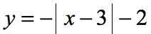
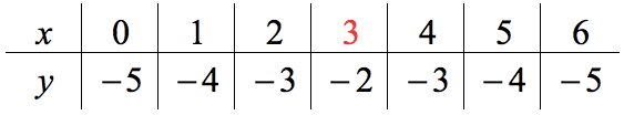
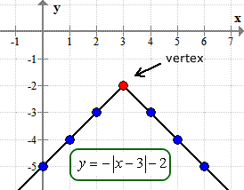
the graph of an absolute value function where the vertex is located in the third quadrant. the point is located at (-3,-4).

Example 4: Graph the absolute value function below using the table of values.

This is an example of an absolute value function whose graph is an inverted “V”. This happens because the coefficient of the absolute value symbol is negative, that is, [latex] – 1[/latex].

Let’s rewrite this in the standard form.

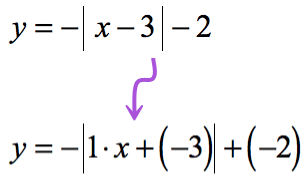
That means [latex]m = 1[/latex], [latex]b = -3[/latex], and [latex]c = -2[/latex].

Solving the vertex of the function,

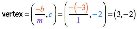
The table of values will have a center value of [latex]x = 3[/latex].

a table with two columns. the x column has entries 0, 1, 2, 3, 4, 5, 6 while the y column has entries -5, -4, -3, -2, -3, -4, -5

Plotting the points in the [latex]xy[/latex]-axis,

the graph of an inverted absolute value function. its vertex is found at (3,-2)

You might also be interested in:

Solving Absolute Value Equations
Solving Absolute Value Inequalities