Graphing a Line using the Slope and [latex]y[/latex]-intercept

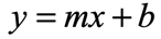
To graph a line using its slope and [latex]y[/latex]-intercept, we need to make sure that the equation of the line is in the Slope-Intercept Form,

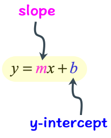
From this format, we can easily read off both the values of the slope and [latex]y[/latex]-intercept. The slope is just the coefficient of variable [latex]x[/latex] which is [latex]m[/latex], while the [latex]y[/latex]-intercept is the constant term [latex]b[/latex].

Here’s a quick diagram to emphasize this idea.

in y=mx+b, m is the slope while b is the y-intercept

When these two pieces of information are identified, we are guaranteed to successfully graph the equation of the line.

How to Graph a Line using the Slope and [latex]y[/latex]-intercept

Plot the [latex]y[/latex]-intercept [latex]\left( {0,b} \right)[/latex] in the [latex]xy[/latex] axis. Remember, this point always lies on the vertical axis [latex]y[/latex].

the point (0,b) is plotted on the xy axis

Starting from the [latex]y[/latex]-intercept, find another point using the slope. Slope contains the direction how you go from one point to another.

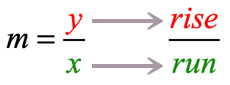
m is equal to y over x or the rise over run

The numerator tells you how many steps to go up or down (rise) while the denominator tells you how many units to move left or right (run).

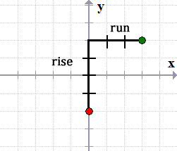
from a given point, the slope gives the instructions how many units to rise and to run

Connect the two points generated by the [latex]y[/latex]-intercept and the slope using a straight edge (ruler) to reveal the graph of the line.

from the y intercept, find another point using the slope then connect the two points with a line

Examples of Graphing a Line using the Slope and [latex]y[/latex]-intercept

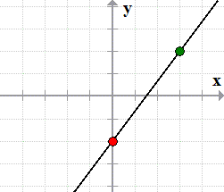
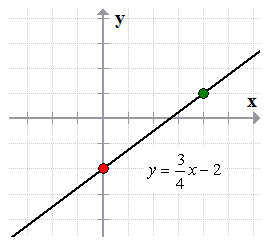
Example 1: Graph the line below using its slope and [latex]y[/latex]-intercept.

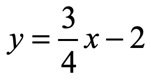
Compare [latex]y = mx + b[/latex] to the given equation [latex]\large{y = {3 \over 4}x – 2}[/latex]. Clearly, we can identify both the slope and [latex]y[/latex]-intercept. The [latex]y[/latex]-intercept is simply [latex]b = – 2[/latex] or [latex]\left( {0,2} \right)[/latex] while the slope is [latex]\large{m = {3 \over 4}}[/latex].

Since the slope is positive, we expect the line to be increasing when viewed from left to right.

Step 1: Let’s plot the first point using the information given to us by the [latex]y[/latex]-intercept which is the point [latex]\left( {0, – 2} \right)[/latex].

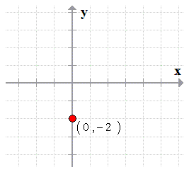
the point (0,-2) is plotted on the xy axis

Step 2: From the [latex]y[/latex]-intercept, find another point using the slope. The slope is [latex]m = {3 \over 4}[/latex], that means, we go up [latex]3[/latex] units and move to the right [latex]4[/latex] units.

from the point (0,-2), move 3 units up and 4 units to the right to get to the other point

Step 3: Connect the two points to graph the line.

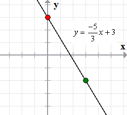
connect the points (0,-2) and (4,1) with a line

Example 2: Graph the line below using its slope and [latex]y[/latex]-intercept.

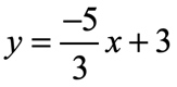
I know that the slope is [latex]\large{m = {{ – 5} \over 3}}[/latex] and the [latex]y[/latex]-intercept is [latex]b = 3[/latex] or [latex]\left( {0,3} \right)[/latex]. Since the slope is negative, the final graph of the line should be decreasing when viewed from left to right.

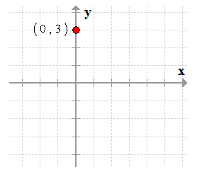
Step 1: Begin by plotting the [latex]y[/latex]-intercept of the given equation which is [latex]\left( {0,3} \right)[/latex].

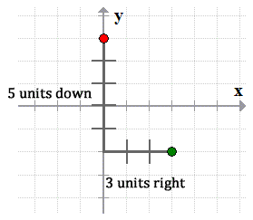
the point (0,3) is plotted on the xy axis

Step 2: Use the slope [latex]\large{m = {{ – 5} \over 3}}[/latex] to find another point using the [latex]y[/latex]-intercept as the reference. The slope tells us to go down [latex]5[/latex] units and then move [latex]3[/latex] units going to the right.

using (0,3) as the starting point, move 5 units down and 3 units to the right to find the other point

Step 3: Draw a line passing through the points.

connect the points (0,3) and (3,-2) with a line

You might also be interested in:

Three Ways to Graph a Line
Graphing a Line using Table of Values
Graphing a Line Using X and Y intercepts